Fine-Tuning Vision Models on Expert Masks: A Guide to SAM, DINO and VLMs

Introduction

Anyone adapting vision foundation models can start from a candid source: the paper that introduced the Segment Anything Model (SAM). Its authors list the model's limits: "It can miss fine structures, hallucinates small disconnected components at times". They say they built it for generality, and they expect domain-specific tools to beat it in their own domains. The Stanford report that named the category made the same point. It defines foundation models as adaptable to many downstream tasks, and its authors chose the term for their "critically central yet incomplete character".

Vision foundation models now cover a lot of ground. SAM 2 segments and tracks objects through video, SAM 3 segments every instance of a named concept, and DINOv3 ships a backbone trained on satellite imagery. Out of the box, they are often good enough for street scenes and product photos. A steel inspector or a geospatial analyst finds the limit quickly: a low-contrast scratch, a road seen from orbit, a small irregular target.

Closing that gap by fine-tuning vision models takes surprisingly little compute. The training data decides the result: which masks you train and test on, and who drew them. This guide explains what vision foundation models are and where they fail on specialist visual data. It compares the main ways to adapt them, shows how vision language models differ, and reviews the evidence on mask quality. It ends with a workflow: the quality engineer or the imagery analyst draws the masks that matter, and the platform measures whether those masks agree.

What Are Vision Foundation Models, and What Were They Trained On?

A vision foundation model is a large image model pretrained on broad data so it can be adapted to many tasks. Two families matter for segmentation work.

The first is the promptable segmenter. You give SAM a click or a box and it returns a mask. Segment Anything was trained on SA-1B, more than 1B masks from 11M images. Most of those masks were not drawn by people. Meta's data engine ran in three stages. First, professional annotators labelled 4.3M masks on 120k images with SAM assisting. A semi-automatic stage then added 5.9M masks on 180k images. Finally, a fully automatic stage produced the 1.1B masks that make up the bulk of the release. In the first stage, the average time per mask fell from 34 to 14 seconds as the model improved.

SAM 2 extended the approach to video. Its SA-V dataset has 50.9K videos and 642.6K masklets (an object's mask across frames). Meta reports that annotation time per frame fell from 37.8 seconds with SAM, used frame by frame, to 4.5 seconds with SAM 2 in the loop. That is an 8.4x speed-up inside its own engine. SAM 3 moves from segmenting one prompted object to segmenting every instance of a named concept, and was trained with 4M unique concept labels. Kili's SAM 3 Data Story breaks down that data engine.

The second family is the feature backbone. DINOv2 is a 1B-parameter vision transformer trained without labels on an automatically curated image set. Its stated goal is "features that work across image distributions and tasks without finetuning". For segmentation, the paper trains only a linear layer on top of frozen features (weights that stay fixed during training). Kili's DINOv2 fine-tuning tutorial walks through that pattern for defect classification. DINOv3 scaled the recipe to 7B parameters and 1.7B images, and Meta released a separate satellite backbone trained on Maxar imagery.

None of these models was trained on your defects or your targets. That is the gap fine-tuning fills.

Where Do Vision Foundation Models Fall Short on Specialist Imagery?

The failure modes are well documented, and they cluster in the same places across domains.

Industrial inspection

Song and colleagues tested zero-shot SAM (used as released, with no extra training) on steel strip, magnetic tile and rail surface defects against specialist models trained on each dataset. On SD-saliency-900, SAM scored a structure measure of 0.668 against 0.884 for the best trained model. The authors found that "SAM can hardly identify the patch defects with extremely low contrast". They also found SAM accurate on slender, small defects, so the problem is contrast and similarity to the background, not size alone.

Researchers who later fine-tuned SAM on about 15,000 real factory anomaly images put it more bluntly. In their words, the original SAM model "lacks the ability to recognize defects". It also tends to segment continuous regions that are not anomalies.

Remote sensing

Overhead imagery has its own pattern. Ren and colleagues tested SAM on a set of widely studied overhead-imagery benchmarks. SAM often generalised well, but "SAM consistently performs very poorly (IoU<10) on the road segmentation task". IoU (intersection over union) measures how much a predicted mask overlaps the true one; here it runs from 0 to 100. Point prompts did much worse than boxes. Osco and colleagues report that "the segmentation of smaller and irregular objects poses difficulties for SAM", whatever the prompt. Accuracy also drops noticeably at resolutions coarser than 30 cm.

The common thread

Medical imaging shows the same profile. MedSAM found SAM had limits on targets with "weak boundaries or low contrast". An evaluation on 19 medical datasets found SAM's IoU ranged from 0.1135 on spine MRI to 0.8650 on hip X-ray.

Low contrast, ambiguous edges, small irregular objects, classes that look like background. A quality engineer or an imagery analyst earns their salary in exactly these places. They decide where a defect ends, or whether a faint linear feature is a road. The model's weak spots are the expert's home ground.

How Does Fine-Tuning Vision Models on Your Own Masks Work?

You can adapt a vision foundation model in several ways. They differ mostly in how much of the model you train and how many masks you need.

‍

‍

PerSAM is the lightest option: it adapts SAM to one object type from one masked example. It suits a recurring part or a single target class. It won't teach SAM what a defect is in general.

Frozen backbones are the default for DINO-class models. Meta's DINOv3 satellite model card recommends frozen features and says of full fine-tuning, "it is recommended to keep this option as a last resort". The canopy-height work by Meta and the World Resources Institute followed that pattern. Its best results came from freezing all layers of the self-supervised encoder and training a decoder against aerial lidar.

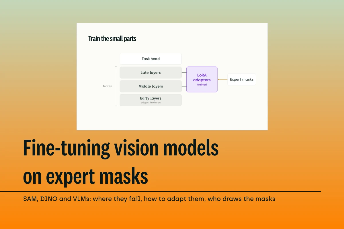
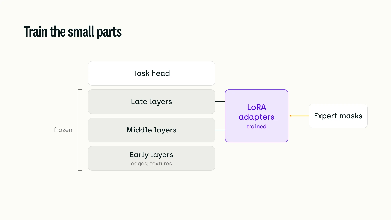
Adapters are where most industrial results sit. SAMed applied LoRA to SAM's image encoder and reached 81.88 Dice (an overlap score between predicted and reference masks, reported here as a percentage) on the Synapse multi-organ segmentation dataset. The factory-image study above used the same family of methods. HQ-SAM kept SAM's weights intact and trained only new components on a dataset of 44K fine-grained masks. Its authors built it because SAM's mask quality falls short on objects with intricate structures.

RSPrompter learns to prompt SAM from the dataset's masks. For remote sensing instance segmentation, that beat both a trained detector feeding SAM and a conventional Mask R-CNN, which scored 54.22 mask AP (average precision over masks). At the far end, MedSAM fine-tuned SAM on its 1,570,263 image-mask pairs. It reached a median Dice of 87.8% on nasopharynx cancer segmentation, a 52.3% improvement over SAM.

Protect what the pre-trained model already knows

Whatever the method, the fine-tuning process carries one constant risk: overwriting what the pre-trained model already does well. The early layers hold the most general features. Yosinski and colleagues found that first-layer features resemble "Gabor filters and color blobs" and "appear not to be specific to a particular dataset or task". Those edge and texture detectors are what you want to keep.

Kumar and colleagues showed what happens when they move. They tested 10 datasets with a distribution shift, where test images differ from training images. On average, full fine-tuning was 2% more accurate than a linear layer on frozen features on images like the training set ("in distribution"). On shifted images ("out of distribution"), it was 7% less accurate. The cause, in their words: "the lower layers of the neural network change simultaneously and distort the pretrained features". Training the linear head first and then fine-tuning everything (LP-FT) beat both. Freezing the backbone, adding adapters and keeping the learning rate small all protect those lower layers.

Augmentation is the other lever. It works best when it copies deployment conditions rather than adding generic variety: the lighting, camera angle and resolution your line or sensor actually produces. Osco's finding that SAM degrades at coarser resolutions is a reminder that resolution is part of the domain.

The pattern across these results: the compute is the cheap part. Four hours on eight GPUs, two trainable parameters, a frozen backbone. What changes from one project to the next is the mask set.

How Do You Fine-Tune a Vision Language Model?

Not every vision model returns a mask. A vision language model (VLM) takes an image and a text input and writes text back. PaliGemma describes this as an "image+text in, text out API", with the prediction generated "in the form of a text string". LLaVA, an early open VLM, connects "a vision encoder and an LLM" (large language model). Its authors fine-tuned it on 158K instruction-following samples. Closed multimodal models such as Google's Gemini work the same way from the user's side. Gemini's technical report describes capabilities "across image, audio, video, and text understanding".

That makes VLMs the natural fit for visual question answering: is there a defect on this weld, or which vehicle types are in this scene?

Try prompt engineering before you fine-tune the model

Instruction-tuned VLMs often answer simple visual questions without any extra training, so prompt engineering is the cheapest first step. Some base models are not built for that. PaliGemma's authors say its pretraining aims at transfer, "not necessarily a model that is usable out of the box". Prompts also have a ceiling. They cannot add new knowledge the pretrained model never saw, such as your defect classes. They also don't reliably make the model answer in a specific way every time. That is when you fine-tune the model.

Format the training dataset as image, query and answer

Supervised fine-tuning for a VLM uses the same shape as the benchmarks that measure it: an image, a question and a reference answer. DocVQA defines 50,000 questions on 12,767 document images, split into 10,194 training images and 1,287 test images. ChartQA pairs charts with "9.6K human-written questions as well as 23.1K questions generated from human-written chart summaries". For specific use cases, the training set is your own images, with the questions your users ask and answers your experts wrote or approved. Hugging Face's TRL library accepts this as an "images" column next to the conversation.

The expert argument from the segmentation sections carries over. In a VLM dataset, the answer is the label. A model trained on vague or inconsistent answers learns to give them.

Use parameter-efficient fine-tuning to fit a large model in GPU memory

Full fine-tuning of a large model updates every weight. It needs the most computational resources and puts the most pressure on the lower layers. Parameter-efficient fine-tuning trains a small set of extra weights instead, significantly reducing what a run costs. LoRA (low-rank adaptation) adds small trainable matrices to a frozen model. On GPT-3 175B, its authors reported it "can reduce the number of trainable parameters by 10,000 times" and GPU memory by 3 times. Quality was on par with or better than full fine-tuning on the models they tested. QLoRA stores the frozen base model in 4-bit precision and trains LoRA adapters on top. That "reduces memory usage enough to finetune a 65B parameter model" on a single 48GB GPU.

The trade-off has been measured for large language models. Biderman and colleagues found that on code and maths, LoRA "substantially underperforms full finetuning" but "better maintains the base model's performance on tasks outside the target domain". Those results come from language model experiments, not VLMs. The question to test on your own task is the same: how much better performance you gain against how much the model loses elsewhere.

Open models such as PaliGemma and LLaVA give you access to the weights. A QLoRA run with TRL looks like this. The model, file names and settings are placeholders, not recommendations.

‍

import torch
from datasets import Dataset
from PIL import Image
from peft import LoraConfig
from transformers import BitsAndBytesConfig
from trl import SFTConfig, SFTTrainer

# One row per (image, query, answer) example, answers written or approved by experts
rows = [
    {
        "images": [Image.open("weld_0412.png")],
        "messages": [
            {"role": "user", "content": "Is there a defect on this weld? If so, what type and where?"},
            {"role": "assistant", "content": "Yes: porosity near the left end of the bead."},
        ],
    },
    # ... more expert-reviewed examples
]
train_dataset = Dataset.from_list(rows)

# QLoRA: load the base model frozen in 4-bit
bnb_config = BitsAndBytesConfig(
    load_in_4bit=True,
    bnb_4bit_quant_type="nf4",
    bnb_4bit_compute_dtype=torch.bfloat16,
)

# LoRA adapters on every linear layer
peft_config = LoraConfig(
    r=16,
    lora_alpha=16,
    lora_dropout=0.05,
    target_modules="all-linear",
    task_type="CAUSAL_LM",
)

args = SFTConfig(
    output_dir="vlm-weld-qa-lora",
    num_train_epochs=3,              # training epochs: check against your expert test set
    per_device_train_batch_size=1,   # batch size per device: lower it first if GPU memory runs out
    gradient_accumulation_steps=8,   # keeps the effective batch size up
    gradient_checkpointing=True,     # lower memory usage, longer training time
    max_length=None,                 # don't truncate image tokens
)

trainer = SFTTrainer(
    model="Qwen/Qwen2.5-VL-3B-Instruct",
    args=args,
    train_dataset=train_dataset,
    peft_config=peft_config,
    quantization_config=bnb_config,
)
trainer.train()
trainer.save_model()  # saves the LoRA adapters, not a full copy of the model

‍

A few settings decide memory usage and training time. Batch size is the first thing to lower when a run doesn't fit on the device. Gradient accumulation adds up several small batches before each weight update, so the effective batch size stays the same. Gradient checkpointing recomputes some intermediate values instead of storing them, which saves memory at the cost of speed. The max_length=None line follows TRL's advice for VLMs, because truncating a sequence can remove image tokens and break training. TRL's default learning rate for SFT (supervised fine-tuning) is 2e-5. The number of training epochs (full passes over the training set) is a choice to validate on held-out expert examples. The saved output is a small set of adapters, so each new model for a new use case sits on top of the same base model.

When shape matters, a text answer is not enough

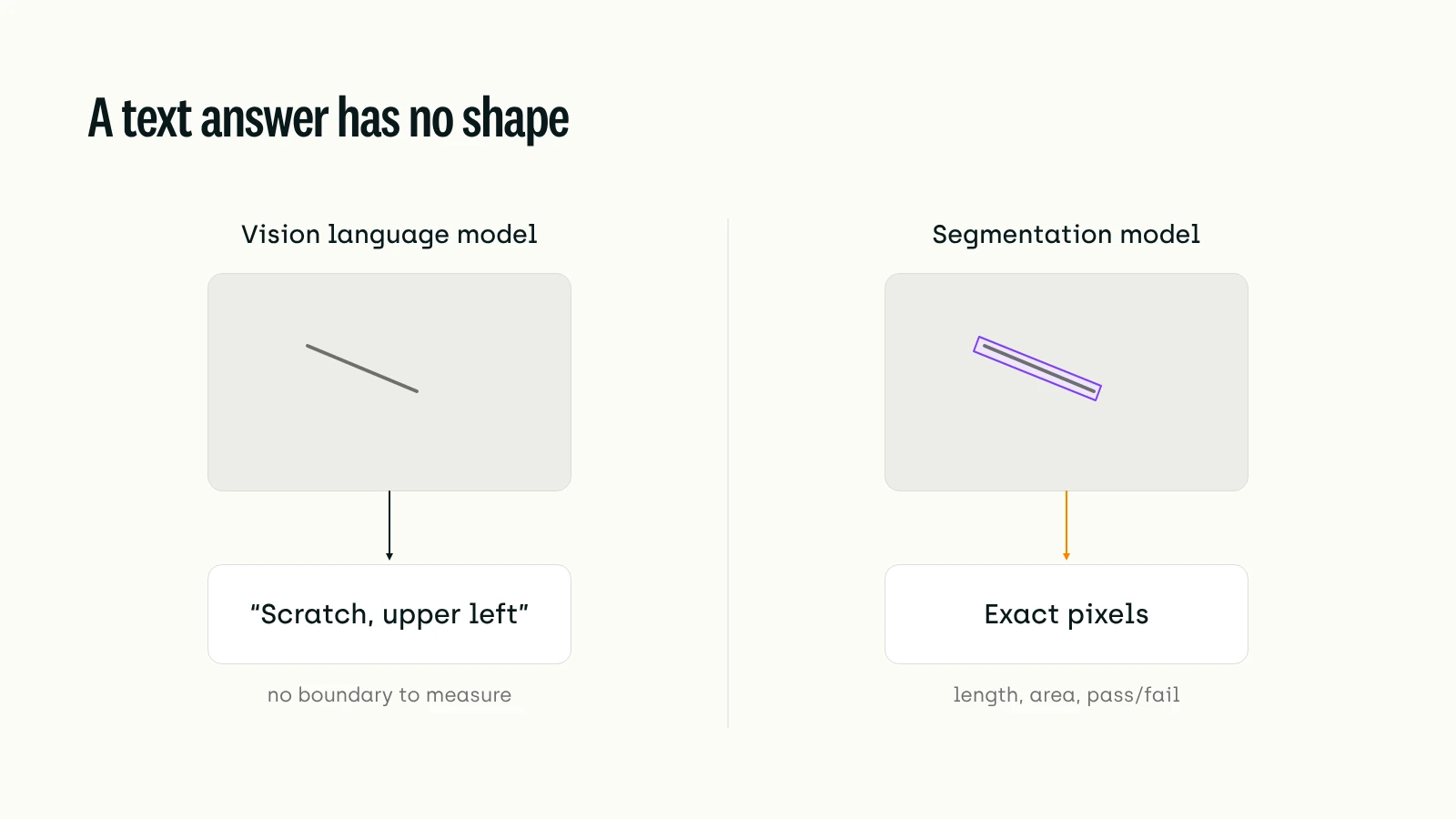
A VLM can tell you a panel has a scratch near the upper-left corner. It cannot tell you the exact pixels the scratch covers. You need those to measure a defect's length or area, apply a pass/fail threshold, or track an object across frames. Which model you need depends on the question, not the image type. The same steel panel can feed a VLM that answers "is there a defect?" and a segmenter that outlines it. When shape matters, every pixel of the mask counts, and so does the person who drew it.

Why Does It Matter Who Draws the Masks?

A fine-tuned model learns the boundary its masks draw. If two annotators would draw a scratch differently, the model is trained on both versions, and your test set scores it against only one of them.

The clearest evidence on annotator quality comes from medical imaging. Rädsch and colleagues studied 14,040 images annotated by 156 professional annotators from four companies and 708 crowdworkers. With minimal text instructions, the professionals' surgical instrument masks reached a median Dice of 0.93, against 0.67 for the crowdworkers. Adding example images to the labelling instructions improved quality; making the text longer did not.

Experts disagree too. When 11 radiologists delineated 3,193 contours on 490 CT slices, the mean volume overlap variability between any two of them ranged from 5% to 57%. Groups of two observers captured 37% of the variability; groups of five, 72%.

Industrial defects have the same property. Niu and colleagues studied noisy labels in surface-defect data. They note that "The boundary between the defect and the background is usually not an absolute line". Similar regions end up labelled differently, depending on each annotator's standards. Errors at the boundary are the ones that hurt. On liver segmentation, Heller and colleagues found that every architecture they tested coped well with label errors away from the boundary. Performance declined steadily as boundary errors grew.

In manufacturing, the person who holds that definition is the quality engineer or line operator. In public sector and defence, it is the imagery or intelligence analyst. Their judgment is what the mask encodes. In the US, the National Geospatial-Intelligence Agency (NGA) announced a call to industry worth more than $700 million for data labelling to train computer vision models. NGA director Vice Adm. Frank Whitworth put the human role plainly: "Data labeling is the process where the human actually identifies the object".

Do You Need Expert Masks for Every Training Image?

No, and the evidence here cuts against the simplest version of the expert argument.

In the Sen1Floods11 flood-mapping dataset, trained remote-sensing analysts hand-labelled 446 chips, and about 4,385 more were labelled automatically. The authors report that "The model trained on hand-labeled data does not provide the best results" on any of their tests. Volume won. On street scenes, Zlateski and colleagues studied convolutional neural networks (ConvNets). They found "the performance of ConvNets mostly depends on the time spent creating the training labels". A larger coarse set can match a smaller fine one. Pretraining on coarse labels and then fine-tuning on a few fine ones matches or beats it, at a fraction of the cost.

Remote sensing also has a dataset built almost without human masks. SAMRS used SAM to turn existing detection boxes into masks, producing 105,090 images and 1,668,241 instances. That buys scale, with masks whose accuracy nobody measured.

Read together, these results say where expert time pays off most:

• The test set. In Sen1Floods11, every model was scored on held-out hand-labelled chips, not on the automatic labels. A model checked against machine masks is checked against the model's own blind spots. Kili's guide to golden datasets covers how to build one.
• The labelling guideline and its example images, which Rädsch showed move quality more than extra text.
• Corrections on the hard cases: the low-contrast patches and small irregular objects where zero-shot SAM fails.

SAM's own data engine already works this way. The model proposes, a person corrects, and per-mask time drops from 34 to 14 seconds. The difference for a domain project is that the person correcting should be the one who knows where the defect ends.

What Does an Expert-Mask Workflow Look Like in Practice?

A workflow that puts expert time where it counts has six steps.

1. Write the mask specification with pictures. Define each class, where its boundary sits, and what to do with ambiguous regions, using annotated example images for each edge case.
2. Have experts draw the test set first. Put every test image in front of at least two experts, measure their agreement, and resolve disagreements before any model sees the data.
3. Let the model draft and the expert correct. Pre-label training images with SAM 2 or your current fine-tuned model, and have experts fix the masks. They should spend most of their time on the regions where the model is weak.
4. Measure the experts as well as the model. Keep a share of training images double-annotated and track agreement per class and per annotator, so a drifting standard shows up before it reaches the model.
5. Adapt the cheapest way first. Try a frozen backbone with a head, or adapters, and score every variant on the expert test set.
6. Send the failures back. The images the adapted model gets wrong become the next batch for expert correction.

Kili's semantic segmentation tool covers steps 2 and 3 for images. Experts can create masks by painting or outlining them with Brush and Lasso, and trim them with Eraser. They can also use interactive segmentation with SAM 2 in two modes: Rapid, the faster default, and High-Res, which is more precise and slower. You can upload existing model masks as predictions for experts to correct through the Python SDK.

For video, the video labelling guide documents SAM 2 smart tracking that follows a segmented object across the next 50 frames. Kili's latest updates extend smart tracking to several objects at once and let Video projects pull assets from cloud storage.

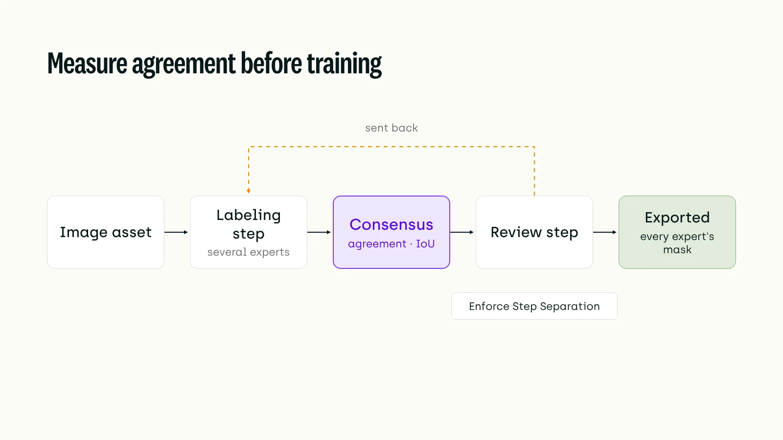
Steps 2 and 4 rely on measurement. You enable consensus on the labelling step by setting a number of labellers and a coverage percentage. Several experts then mask a chosen share of assets in parallel, without seeing each other's annotations. For semantic segmentation, the consensus score is intersection over union, per the calculation rules. A workflow can add several review levels, with Enforce Step Separation on by default so no one reviews their own masks. Reviewers send a masked asset back to its labeller through the workflow's send-back step. When you export, choosing the latest label from each author keeps every expert's mask, so the disagreement itself becomes data for your test set.

The Mask Specification Is the Model Specification

Each generation of vision foundation models is larger and covers more. DINOv3 has 7B parameters, and SAM 3 segments every instance of a named concept. What these models cannot absorb from more pretraining is your definition of a defect, a road at your resolution, or a target class your analysts care about. That definition lives in the masks.

As adaptation gets cheaper, the expert-drawn test set stops being a final check and becomes the asset that outlasts any single model. Some teams keep that test set, measure the agreement behind it, and route the model's failures back to the same experts. They can score the next backbone against the same reference the week it ships. Teams that trained on unmeasured masks will have to find out what their model learned the hard way.

Resources

Vision foundation models

• On the Opportunities and Risks of Foundation Models – Bommasani et al., Stanford CRFM, 2021 (preprint)
  • https://arxiv.org/abs/2108.07258
• Segment Anything – Kirillov et al., ICCV 2023 (Meta; dataset figures self-reported)
  • https://ar5iv.labs.arxiv.org/html/2304.02643
• SAM 2: Segment Anything in Images and Videos – Ravi et al., ICLR 2025 (Meta; annotation-time figures self-reported)
  • https://arxiv.org/html/2408.00714
• SAM 3: Segment Anything with Concepts – Carion et al., Meta, 2025 (preprint, self-reported)
  • https://arxiv.org/abs/2511.16719
• DINOv2: Learning Robust Visual Features without Supervision – Oquab et al., TMLR 2024
  • https://arxiv.org/abs/2304.07193
• DINOv3: Self-supervised learning for vision at unprecedented scale – Meta AI blog, 14 Aug 2025 (self-reported)
  • https://ai.meta.com/blog/dinov3-self-supervised-vision-model/
• facebook/dinov3-vitl16-pretrain-sat493m – Meta AI model card, Hugging Face (self-reported)
  • https://huggingface.co/facebook/dinov3-vitl16-pretrain-sat493m

Zero-shot limits on specialist imagery

• SAM Era: Can It Segment Any Industrial Surface Defects? – Song et al., Computers, Materials & Continua, 2024
  • https://www.sciencedirect.com/org/science/article/pii/S1546221824003394
• Promptable Anomaly Segmentation with SAM Through Self-Perception Tuning – Yang et al., 2024 (preprint)
  • https://arxiv.org/html/2411.17217
• Segment Anything, From Space? – Ren et al., WACV 2024
  • https://openaccess.thecvf.com/content/WACV2024/html/Ren_Segment_Anything_From_Space_WACV_2024_paper.html
• The Segment Anything Model (SAM) for Remote Sensing Applications: From Zero to One Shot – Osco et al., International Journal of Applied Earth Observation and Geoinformation, 2023
  • https://ar5iv.labs.arxiv.org/html/2306.16623
• Segment Anything Model for Medical Image Analysis: An Experimental Study – Mazurowski et al., Medical Image Analysis, 2023
  • https://arxiv.org/abs/2304.10517

Fine-tuning and adaptation

• Segment Anything in Medical Images (MedSAM) – Ma et al., Nature Communications, 2024
  • https://pmc.ncbi.nlm.nih.gov/articles/PMC10803759
• Personalize Segment Anything Model with One Shot – Zhang et al., 2023 (preprint)
  • https://arxiv.org/abs/2305.03048
• Very High Resolution Canopy Height Maps from RGB Imagery – Tolan et al., Remote Sensing of Environment, 2024
  • https://arxiv.org/abs/2304.07213v3
• Customized Segment Anything Model for Medical Image Segmentation (SAMed) – Zhang & Liu, 2023 (preprint)
  • https://arxiv.org/abs/2304.13785
• Segment Anything in High Quality (HQ-SAM) – Ke et al., NeurIPS 2023
  • https://arxiv.org/abs/2306.01567
• RSPrompter: Learning to Prompt for Remote Sensing Instance Segmentation – Chen et al., IEEE TGRS, 2024
  • https://arxiv.org/html/2306.16269v1
• How Transferable Are Features in Deep Neural Networks? – Yosinski et al., NeurIPS 2014
  • https://arxiv.org/abs/1411.1792
• Fine-Tuning can Distort Pretrained Features and Underperform Out-of-Distribution – Kumar et al., ICLR 2022
  • https://arxiv.org/abs/2202.10054

Vision language models and parameter-efficient fine-tuning

• PaliGemma: A versatile 3B VLM for transfer – Beyer et al., Google DeepMind, 2024 (preprint)
  • https://arxiv.org/abs/2407.07726
• Visual Instruction Tuning (LLaVA) – Liu et al., NeurIPS 2023
  • https://arxiv.org/abs/2304.08485
• Gemini: A Family of Highly Capable Multimodal Models – Gemini Team, Google, 2023 (technical report, self-reported)
  • https://arxiv.org/abs/2312.11805
• DocVQA: A Dataset for VQA on Document Images – Mathew et al., WACV 2021
  • https://arxiv.org/abs/2007.00398
• ChartQA: A Benchmark for Question Answering about Charts with Visual and Logical Reasoning – Masry et al., Findings of ACL 2022
  • https://arxiv.org/abs/2203.10244
• LoRA: Low-Rank Adaptation of Large Language Models – Hu et al., ICLR 2022
  • https://arxiv.org/abs/2106.09685
• QLoRA: Efficient Finetuning of Quantized LLMs – Dettmers et al., NeurIPS 2023
  • https://arxiv.org/abs/2305.14314
• LoRA Learns Less and Forgets Less – Biderman et al., TMLR 2024
  • https://arxiv.org/abs/2405.09673
• SFT Trainer – TRL documentation, Hugging Face
  • https://huggingface.co/docs/trl/sft_trainer

Mask quality and annotators

• Labelling Instructions Matter in Biomedical Image Analysis – Rädsch et al., Nature Machine Intelligence, 2023
  • https://link.springer.com/article/10.1038/s42256-023-00625-5
• Inter-observer Variability of Manual Contour Delineation of Structures in CT – Joskowicz et al., European Radiology, 2019
  • https://cris.huji.ac.il/en/publications/inter-observer-variability-of-manual-contour-delineation-of-struc/
• Learning Trustworthy Model from Noisy Labels Based on Rough Set for Surface Defect Detection – Niu et al., 2023 (preprint)
  • https://arxiv.org/html/2301.10441v1
• Imperfect Segmentation Labels: How Much Do They Matter? – Heller et al., 2018 (preprint)
  • https://arxiv.org/abs/1806.04618
• Sen1Floods11: A Georeferenced Dataset to Train and Test Deep Learning Flood Algorithms for Sentinel-1 – Bonafilia et al., CVPR Workshops 2020
  • https://openaccess.thecvf.com/content_CVPRW_2020/papers/w11/Bonafilia_Sen1Floods11_A_Georeferenced_Dataset_to_Train_and_Test_Deep_Learning_CVPRW_2020_paper.pdf
• On the Importance of Label Quality for Semantic Segmentation – Zlateski et al., CVPR 2018
  • https://openaccess.thecvf.com/content_cvpr_2018/html/Zlateski_On_the_Importance_CVPR_2018_paper.html
• SAMRS: Scaling-up Remote Sensing Segmentation Dataset with Segment Anything Model – Wang et al., NeurIPS 2023 Datasets and Benchmarks
  • https://papers.nips.cc/paper_files/paper/2023/hash/1be3843e534ee06d3a70c7f62b983b31-Abstract-Datasets_and_Benchmarks.html

Industry context

• NGA slates $700M for AI data labeling, launches standard model push – Theresa Hitchens, Breaking Defense, 3 Sep 2024
  • https://breakingdefense.com/2024/09/nga-slates-700m-for-ai-data-labeling-launches-standard-model-push/

Kili Technology

• Data Story: SAM 3 – Kili Technology blog
  • https://kili-technology.com/blog/sam-3-data-story
• DINOv2 Fine-Tuning Tutorial – Kili Technology blog
  • https://kili-technology.com/blog/dinov2-fine-tuning-tutorial-maximizing-accuracy-for-computer-vision-tasks
• How to Build Golden Datasets for Testing, Fine-tuning, and Evaluating AI Models – Kili Technology blog
  • https://kili-technology.com/blog/how-to-build-golden-datasets-for-testing-fine-tuning-and-evaluating-ai-models
• Using semantic segmentation – Kili documentation
  • https://docs.kili-technology.com/docs/semantic-segmentation
• How to import segmentation pre-annotations – Kili Python SDK tutorial
  • https://python-sdk-docs.kili-technology.com/26.1/sdk/tutorials/pixel_level_masks
• Labeling video assets – Kili documentation
  • https://docs.kili-technology.com/docs/labeling-video-assets
• Changelog – Kili documentation
  • https://docs.kili-technology.com/changelog
• Calculation rules for quality metrics – Kili documentation
  • https://docs.kili-technology.com/docs/calculation-rules-for-quality-metrics
• Workflow configuration – Kili documentation
  • https://docs.kili-technology.com/docs/workflow-configuration
• Exporting project data – Kili documentation
  • https://docs.kili-technology.com/docs/exporting-project-data
• Contact Kili Technology
  • https://kili-technology.com/contact