AI Summary
Introduction
Object detection is today at the heart of technological concerns as its possibilities and applications are so vast. This field has experienced rapid growth in recent years with the appearance of increasingly efficient models and frameworks such as YoloV5 and Detectron2.
The results obtained are now convincing. Now the research is more and more oriented toward finding a procedure that works with few examples. How do these architectures work? And what are the most promising avenues to make them sample efficient?
Object detection basic functioning
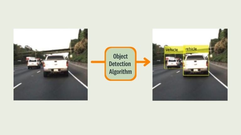
Object detection aims to detect instances of object categories on images. Thus, many approaches can be described the following way: an unlabeled input image that is processed by object detection algorithm to output the labeled image.

Figure 1: Basic object detection model functioning
The main question is: How does the algorithm detect the right objects?
It proceeds in a similar fashion as human beings. It learns by example. In the classical approach, model training algorithms are fed with a large, labeled set of examples (labeled images) on which it will learn a representation of the various categories they belong to.

Figure 2: Classic approach principle
The training phase is critical to modern approaches, but unfortunately, it's also the most resource-consuming and time-consuming one. However, if one wants to adapt the model quickly to a dataset, he needs to reduce the training time. Hence, few-shot object detection approaches come into play.
Few-shot object detection
While the classical approach leverages a large amount of training data, the few-shot approaches involve a small volume thereof: from 1 to 30 examples per category.

Figure 3: Few-shot principle
Such an approach could bring a lot of value to smart annotation procedure and especially improve the annotation experience. Let's introduce a typical workflow based on few-shot object detection to illustrate that.
Let's suppose we have a labeler who wants to annotate a large object detection dataset on an annotation platform like Kili. He/She will only have to annotate a subset of the entire dataset, let's say 10 examples per category. (Figure 4)

Figure 4: Use case – Annotation phase
Then few-shot model will be trained with the examples that the labeler already annotated. (Figure 5)
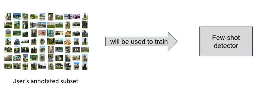
Figure 5: Use case – training phase
Finally, the trained few-shot detector will be used to pre-annotate the rest of the initial dataset and accelerate the annotation of the dataset.

Figure 6: Use case – Pre-annotation phase
Such a tool represents a significant time saving for the users and can make the annotation procedure faster.
The approach considered
As said before, the few-shot principle is to train a model with a small set of examples. Thus, it is legitimate to ask how to obtain a model with comparable efficiency to the classical approaches with so few examples. Let's talk about the transfer learning approach that can be considered as a baseline.
Quick side note on transfer learning principle
So, let's consider that we want to train a model to predict the car's safe stopping distance according to the speed. We will follow the classical training method of training by randomly initializing (Figure 7) a model and then train it to fit the theoretical ideal (2).
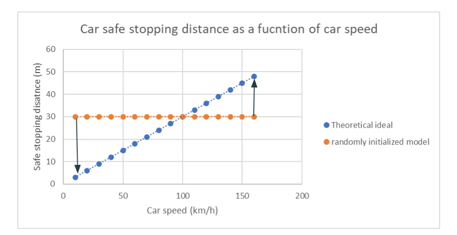
Figure 7: Car safe stopping distance as a function of car speed with randomly initialized model

Figure 8: Car safe stopping distance as a function of car speed with trained model
We now have an efficient model to predict the car's safe stopping distance. However, what we would do to obtain a model which predicts truck safe stopping distance. We can naively reproduce the procedure we followed for the car. However, we can also notice that car safe stopping distance and truck safe stopping distance should follow similar principles.

Figure 9: Car/Truck stopping distance
We intuitively understand that it could be interesting to transfer the knowledge we learn from car to truck situation and then just adjust our model a little bit. Well, that's what transfer learning is all about.
To summarize, the goal of transfer learning is to transfer knowledge from a source domain (large, labeled dataset) to a target domain (smaller). In our example, the source domain is the car stopping distance data, and the target domain is the truck one.
Fine-tuning approach
Similarly to the car/truck transfer example, the fine-tuning approach relies on two steps. First, the base-training phase, during which the entire model will be trained on a large, labeled object detection dataset (source domain). Then, a few-shot fine-tuning phase during which the model's last layers will be fine-tuned on the much smaller target domain dataset.
Fine-tuning is a transfer learning method that aims to take and adjust a model trained on a task to make it perform on another similar task.
Before getting into details of the model architecture and functioning, let's have a look at the two datasets used.
Source dataset
The source dataset must be large i.e it should contain as many object categories and instances as possible. COCO dataset (https://cocodataset.org/#home ) meets these criteria with more than 200 000 labeled images, 80 categories and about 1.5 million object instances.
Target dataset
Plastic-in-river dataset (https://huggingface.co/datasets/Kili/plastic_in_river) has been used as target dataset. It contains four object categories and more than 3000 labeled images. However, only a subset containing 10-shot per category will be considered during the training phase.
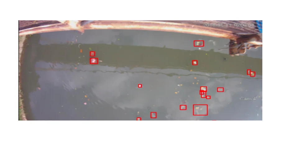
Figure 10: labeled sample from plastic-in-river dataset
The following part will go into the model's technical details and the training procedure.
Base-training phase
Model architecture is a Faster R-CNN based followed by box predictor.
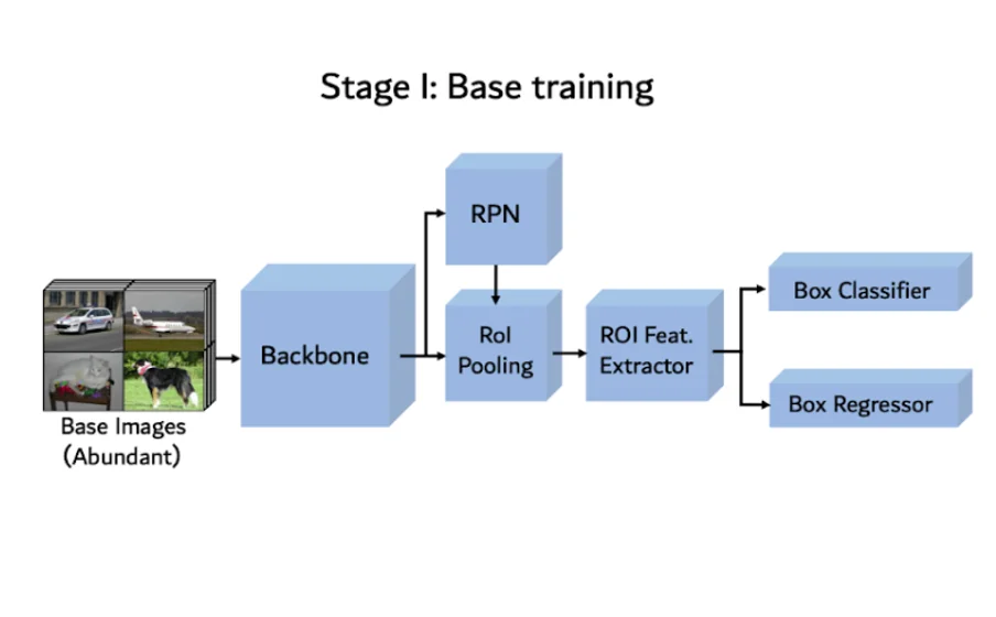
Figure 11: Model architecture – Base training phase
Faster R-CNN architecture is composed of a Backbone (ResNet-101 architecture), Region Proposal Network (RPN), which aims to identify regions in image which contain objects (these regions are so-called proposals). Then there is the Region of interest Pooling. His role is to extract the right features from the backbone based on RPN proposals.
Finally, there is the box predictor composed of a Box classifier and a box regressor. The box regressor predicts the coordinates of the bounding boxes on the image, whereas the box classifier predicts the category of the bounding box object.
Concerning the training, SGD optimizer is used with a learning rate of 0.02, and the training stops when validation loss increases over two consecutive epochs.
Fine-tuning phase
The Faster R-CNN weights will be frozen: they won't be modified at all during this phase, so only box predictor weights will be tuned.
The target dataset will be a subset containing 10-shot per base and novel category.
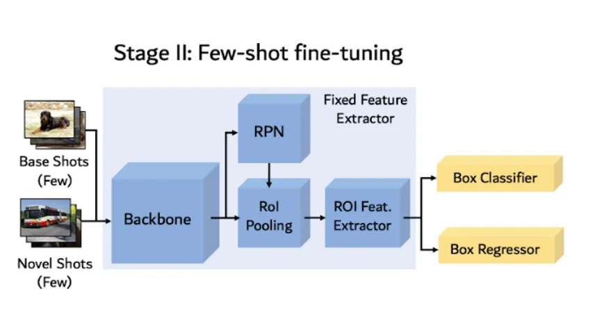
Figure 12: Model architecture – few-shot fine-tuning phase
The training phase is relatively similar to the base training phase except concerning the learning rate, which will be decreased. The reason is intuitive. The pre-trained weights are already good; thus we only want to adjust them and not distort them.
Learn more!
Discover how training data can make or break your AI projects, and how to implement the Data Centric AI philosophy in your ML projects.
Dataset similarities
Transfer learning approach aims to transfer knowledge from a large source domain to a smaller target domain. However, what if the two domains are drastically different? Is it more important to have a medium source dataset highly similar to target one or a larger general dataset?
Experiments of Brad Dwyer on mask-wearing task showed interesting results about that. He used a YoloV5 model base-trained on three different datasets. First, Microsoft COCO, a very large and general dataset containing millions of object instances. Second, WIDER FACE, a smaller one which contains 16,000 images of labeled faces. Finally, BCCD, a blood cell dataset.
Then, he fine-tuned each pre-trained model with a small dataset of face wearing mask and one face not wearing a mask.
He obtains the following results:
Source datasetPrecisionMS COCO50.8%WIDER FACE64.3%BCDD41.6%
Figure 13: Models precision on test face wearing mask test set (https://blog.roboflow.com/transfer-learning-similarity/)
Even if MS COCO is twenty times larger than WIDER FACE, the precision is worse. The fact is that COCO is a general object detection dataset, whereas WIDER FACE is face-specific. This shows that the source dataset choice is critical and how it can impact the efficiency of the final model.
Conclusion
The integration of such a tool would bring value to the customer helping him to annotate data faster. However, the previous results on the similarity of datasets show a limit to this approach. Using a single base dataset (large and general) is less efficient than a specific but more restricted dataset. Thus, it is necessary to rectify the initial approach.
To optimize few-shot detection tasks, there should be a collection of models pre-trained on various specific datasets. Then, each fine-tuning task should be done on the specific model which base domain corresponds the most to the target dataset.
An article by Hugo Degeorges.

.png)
_logo%201.svg)


